How to Freeze Rows and Columns in Excel

Microsoft Excel helps you to organize and analyze extensive data with its spreadsheet software. It plays a vital role starting from a small-scale industry to a large-scale industry. The users can perform financial analysis with this powerful data organization tool. It offers a heap of applications like business analysis, people management, program management, strategic analysis, administration purposes, operation control, and performance reporting. However, it is mainly used to store and sort data for easy analysis. Microsoft Excel 2016 and 2019 support a feature by which you can freeze a row in or a column in Excel. Hence, when you scroll up or down, the frozen panes remain in the same place. This comes in handy when you have data covering multiple rows and columns. Today, we will discuss how to freeze or unfreeze rows, coulumns or panes in MS Excel.

How to Freeze/Unfreeze Rows or Columns in MS Excel

1048576 rows & 16,384 columns in Excel can store an excessive collection of data in an organized manner. Some other exciting features of Excel include:

• Data filtering,
• Data sorting,
• Find and replace feature,
• Built-in formulae,
• Pivot table,
• Password protection, and many more.

Moreover, you can freeze multiple rows or columns in excel. You can freeze a portion of the sheet viz row, column or panes in Ecel to keep it visible while you scroll through the rest of the sheet. This is useful for checking out the data in other parts of your worksheet without losing your headers or labels. Keep reading to learn how to freeze or unfreeze rows, columns or panes in Microsoft Excel.

Important Terminology Before You Begin

• Freeze Panes: Based on the current selection, you can keep the rows and columns visible while the rest of the worksheet scrolls up and down.
• Freeze Top Row: This feature will be helpful if you want to freeze only the first header/top row. This option will keep the top row visible, and you can scroll through the rest of the worksheet.
• Freeze First Column: You can keep the first column visible while you can scroll through the rest of the worksheet.
• Unfreeze Panes: You can unlock all the rows and columns to scroll through the entire worksheet.

Option 1: How to Freeze a Row in Excel

You can freeze a row in Excel or freeze multiple rows in Excel by following the below-mentioned steps:

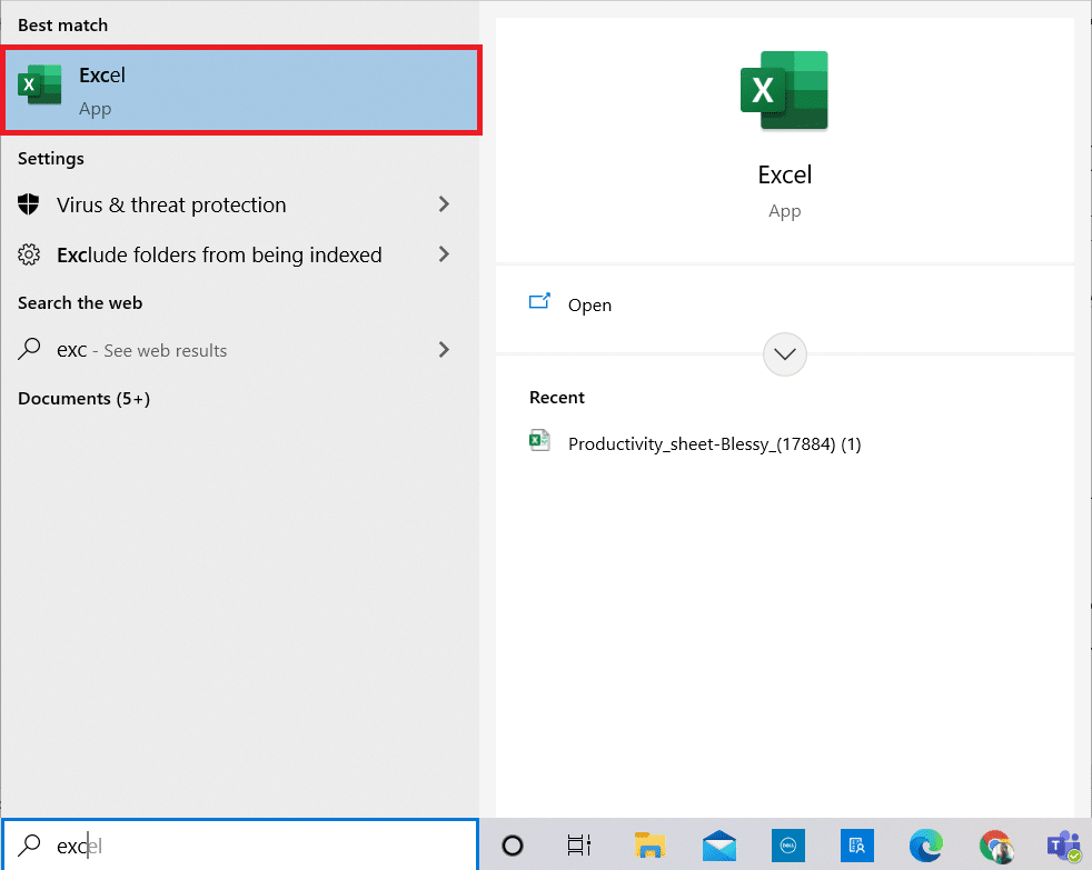
1. Press the Windows key. Type & search Excel and click on it to open it.

2. Open your desired Excel sheet and select any row.

Note 1: Always choose the row that is below the row you want to freeze. This means if you want to freeze up to the 3rd row, you must select the 4th row.

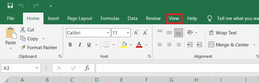
3. Then, select View in the menu bar as shown.

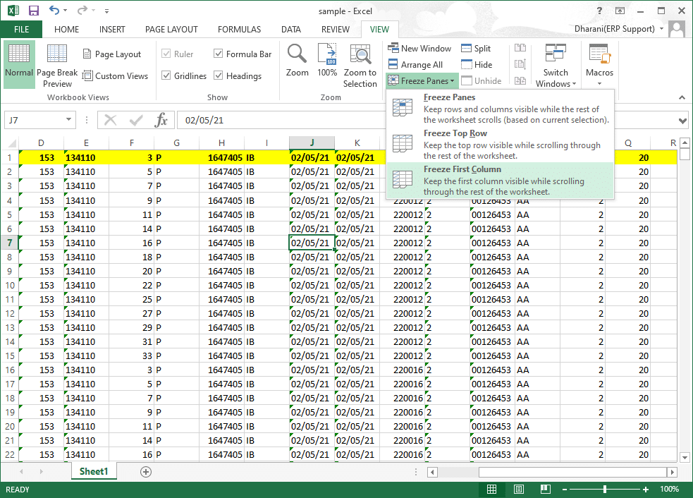
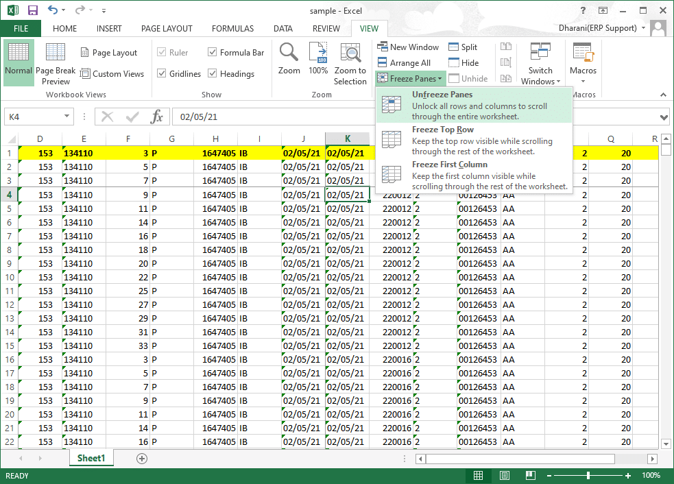
4. Click Freeze Panes > Freeze Panes in the drop-down menu as depicted below.

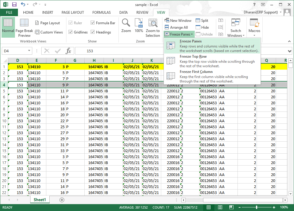
All the rows below the selected row will be frozen. The rows above the selected cell/row will stay in the same place when you scroll down. Here in this example, when you scroll down, row 1, row 2, row 3 will remain in the same place and the rest of the worksheet scrolls.

Also Read: How to Copy and Paste Values Without formulas in Excel

Option 2: How to Freeze Top Row in Excel

You can freeze the header row in the worksheet by following the given steps:

1. Launch Excel as earlier.

2. Open your Excel sheet and select any cell.

3. Switch to the View tab at the top as shown.

4. Click Freeze Panes > Freeze Top Row as shown highlighted.

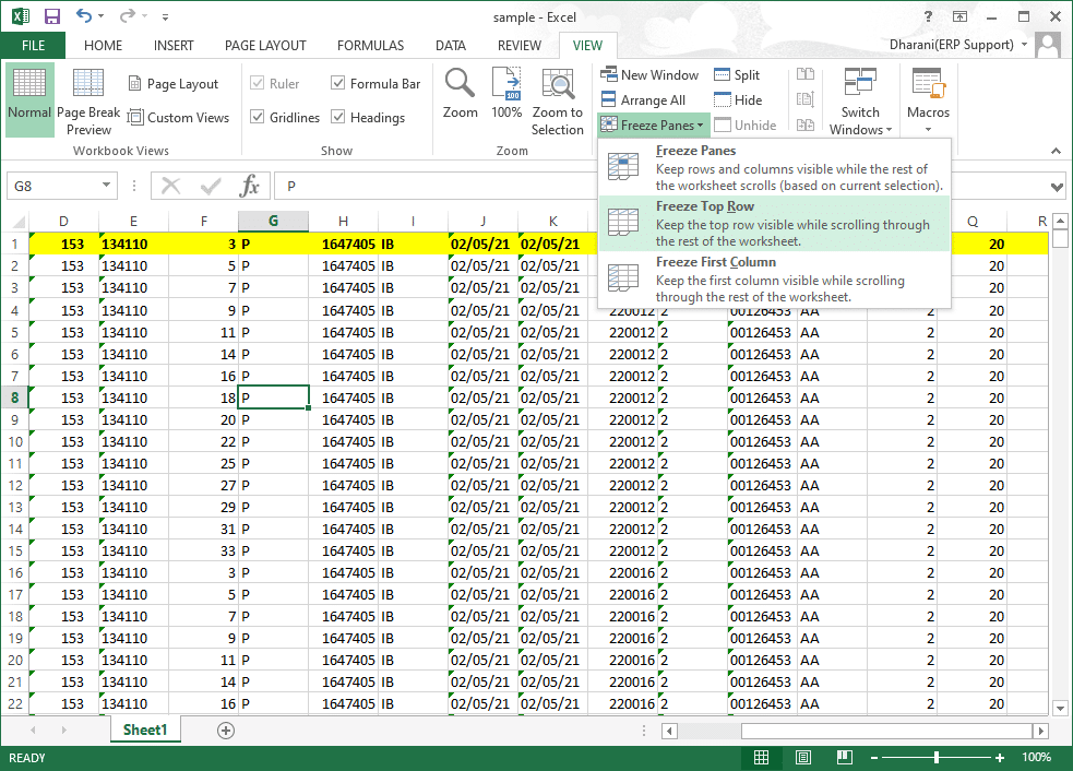
Now, the first top row will be frozen, and the rest of the worksheet will scroll normally.

Also Read: Fix Outlook App Won’t Open in Windows 10

Option 3: How to Freeze a Column in Excel

You can freeze, unfreeze or move multiple columns or a single column in Excel as follows:

1. Press the Windows key. Type & search Excel and click on it to open it.

2. Open your Excel sheet and select any column.

Note: Always choose the column that is right to the column you wanted to freeze. This means that if you want to freeze column F, select column G and so on.

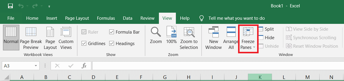
3. Switch to the View tab as shown below.

4. Click Freeze Panes and select Freeze Panes option as depicted.

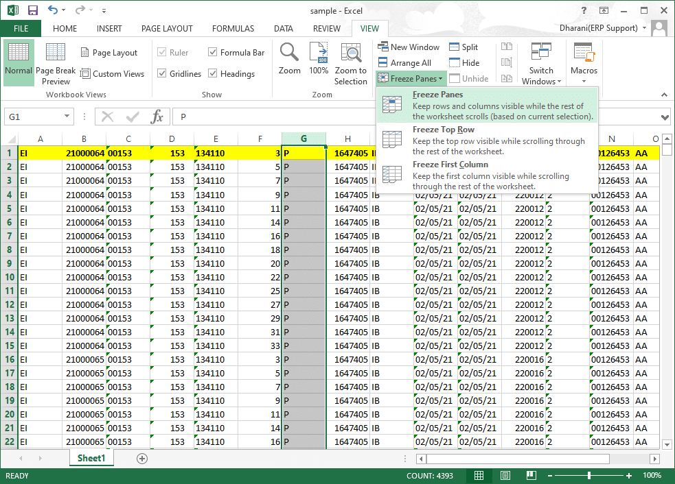
All the columns left of the selected column will be frozen. When you scroll right, the rows in the left of the selected column will stay in the same place. Here in this example, when you scroll right, column A, column B, column C, column D, column E, and column F will stay in the same place, and the rest of the worksheet will scroll left or right.

Option 4: How to Freeze First Column in Excel

You can freeze a column in Excel, i.e., freeze the first column in the worksheet by following the below steps.

1. Launch Excel as earlier.

2. Open your Excel sheet and select any cell.

3. Switch to the View tab from the top as shown.

4. Click Freeze Panes and this time, select Freeze First Column option from drop-down menu.

Thus, the first column will be frozen, where you can scroll through the rest of the worksheet normally.

Also Read: Fix Microsoft Office Not Opening on Windows 10

Option 5: How to Freeze Panes in Excel

For instance, if you are entering data in a report card containing students’ names and marks, it is always a hectic job to scroll to the header (containing subject names) and the label (including the name of students) often. In this scenario, freezing both the row and column fields will help you. Here’s how to do the same:

1. Launch Excel as earlier. Open desired worksheet and select any cell.

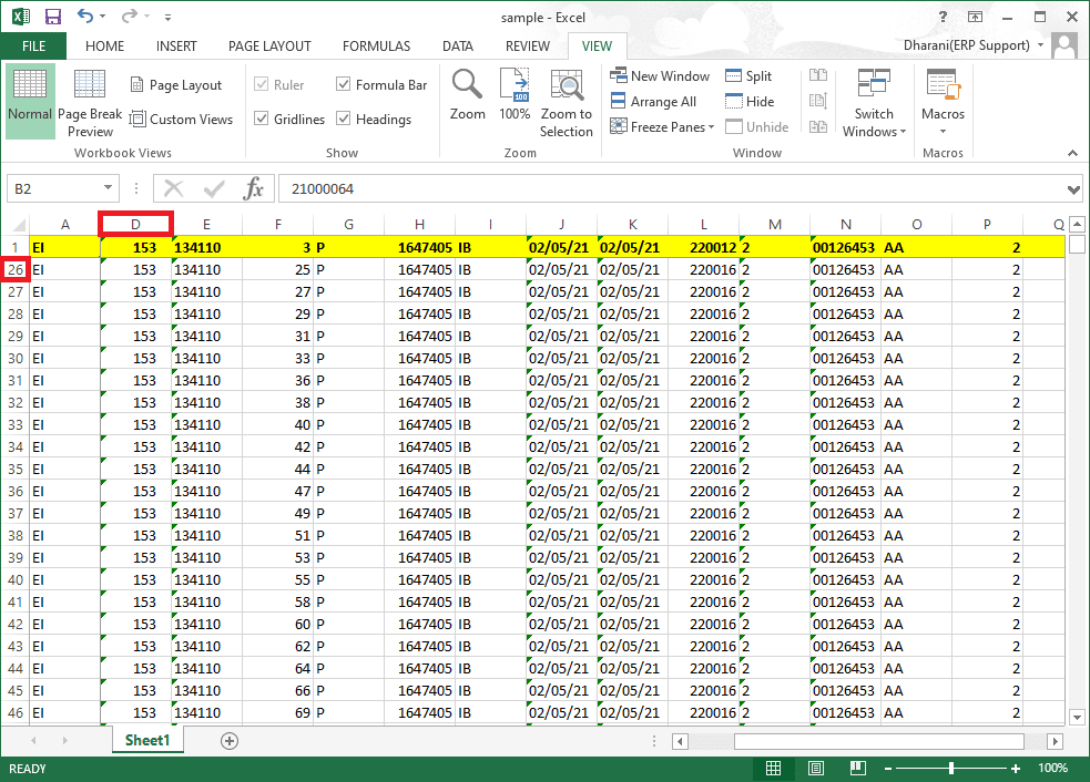
Note 1: Always ensure that you choose a cell to the right of the column and below the row you want to freeze. For example, if you want to freeze the first row & first column, select the cell to the right of the first column pane and below the first-row pane, i.e., select B2 cell.

2. Click on the View tab from the top ribbon.

3. Click Freeze Panes as shown.

4. Select option marked Freeze Panes as illustrated below.

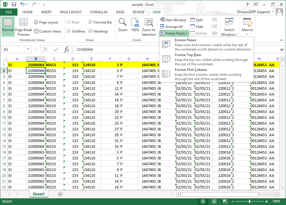
All the rows above the selected row and all the columns to the left of the selected column will be frozen, and the rest of the worksheet scrolls. So here, in this example, the first row and the first column are frozen, and the rest of the worksheet scrolls as depicted below.

How to Unfreeze Rows, Columns, or Panes in Excel

If you have frozen any rows, columns, or panes, you cannot perform another freezing step unless it is removed. To unfreeze rows, columns, or panes in Excel, implement these steps:

1. Select any cell in the worksheet.

2. Navigate to the View tab.

3. Now, select Freeze Panes and click on Unfreeze Panes as depicted below.

Note: Make sure you have any cell/row/column in a frozen state. Otherwise, an option to Unfreeze Panes will not appear.

Also Read: How to Stop Microsoft Teams from Opening on Startup

Pro Tip: How to Create Magic Freeze Button

You can also create a magic freeze/unfreeze button in the Quick Access toolbar to freeze a row, column, first column, first row, or panes with a single click.

1. Launch Excel as earlier.

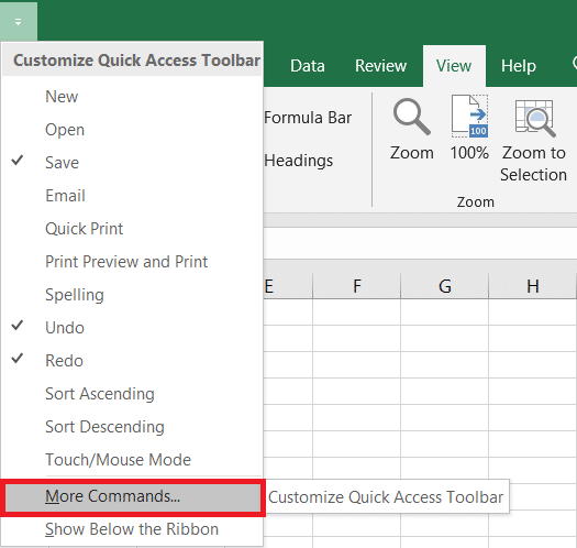
2. Click the down arrow, shown highlighted, from the top of the worksheet.

3. Click More Commands as shown.

4. Select Freeze Panes in the list and then click Add.

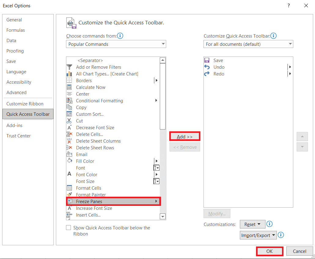
5. Finally, click OK. Freeze Panes Quick Access option will be available at the top of the worksheet in MS Excel.

Frequently Asked Questions (FAQs)

Q1. Why is the Freeze Panes option greyed out in my worksheet?

Ans. The option Freeze Panes is greyed out when you are in editing mode or worksheet is protected. To exit the editing mode, press Esc key.

Q2. How can I lock cells in Excel instead of freezing them?

Ans. You can use the Split option in the View menu to split and lock cells. Alternately, you can create a table by Ctrl + T. Creating a table will lock the column header when you scroll down. Read our guide on How To Lock Or Unlock Cells In Excel.

Recommended:

We hope that this guide was helpful, and you were able to freeze and unfreeze rows, columns or panes in Excel. Feel free to reach out to us with your queries and suggestions via comments section below.