How to INDEX MATCH Multiple Criteria in Google Sheets
Google Sheets is an essential tool that helps you keep a track of things in all walks of life be it personal or professional. There might be times when you have come across situations that require you to find a value from a different table or a sheet. Plenty of functions in Google Sheets allow you to easily find values using different functions. One of these functions is the INDEX MATCH. If you have no idea about this, then don’t worry as this article is going to be the perfect guide for you. In this article, you will learn about how to INDEX MATCH multiple criteria Google Sheets.

How to INDEX MATCH Multiple Criteria in Google Sheets
Here, we have shown the steps to Index Match multiple criteria in Google Sheets.
What is INDEX MATCH?
INDEX Match is one of the functions of Google Sheets that enables users to look for values within the Sheet or other Sheets. This function is also considered the best alternative to other functions like VLOOKUP, HLOOKUP, and LOOKUP. If you didn’t know Both INDEX and MATCH are different functions with limited applications. When combined it enables you to save time and energy by finding complex data values within seconds.
INDEX MATCH multiple criteria syntax Google Sheets starts with the formula of the INDEX function. Match function substitute for the position argument in the formula. The syntax of the INDEX MATCH with multiple criteria is
=INDEX (reference,MATCH(1,(criteria1)*(criteria2)*(criteria3),0))
The syntax of Index Match stands for:
- reference: It is the range of cells from where you will get the target value.
- MATCH: It finds the position of the search key.
- 1: It identifies a particular search key.
- (criteria1)*(criteria2)*(criteria3): It refers to the criteria which are required to be matched.
- 0: It stands for finding the exact value.
Also Read: How to add multiple lines in one cell in Google Sheets
How to INDEX MATCH Multiple Criteria in Google Sheets?
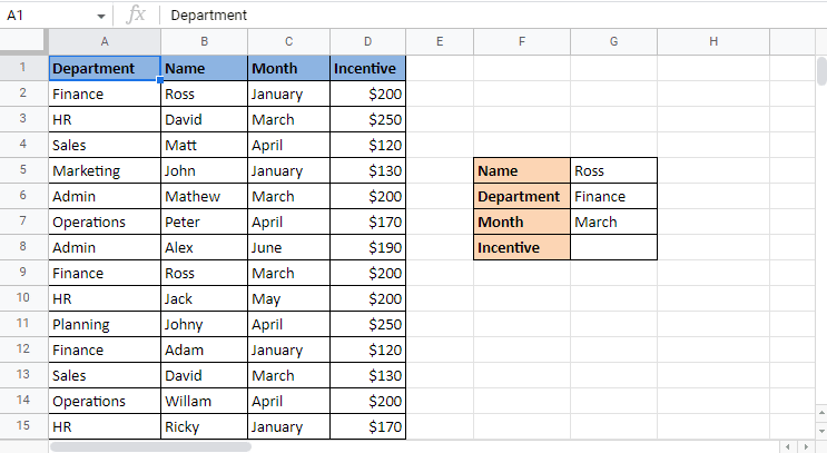
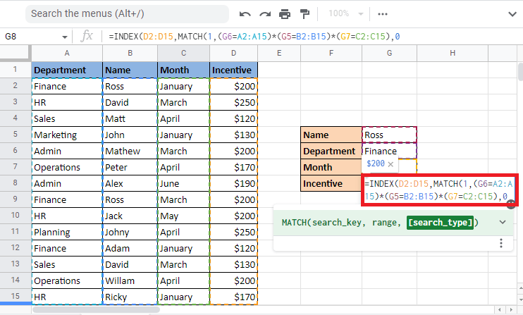
Using INDEX MATCH to find values using multiple criteria in Google Sheets is one of the easy and convenient ways. Read through the article to find out how INDEX MATCH works. This is the data that we are going to use. It contains details of Employees of a company and the incentives they received over the months.
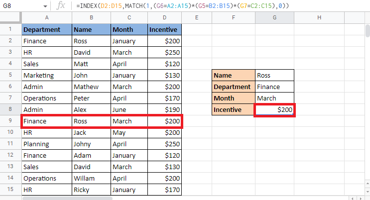
This data consists of various criteria like Employee name, department, month, and incentive. The value we have to find out is the incentive of Ross that he received in March. Now, the confusing part is that Ross from finance has received the incentive twice. How will the function identify which month incentive detail you are looking for? Here the INDEX MATCH function comes into play. Follow the below-mentioned steps to see INDEX match multiple criteria Google Sheets. Further in the article, you will also read about whether you can use INDEX match across multiple Google Sheets.
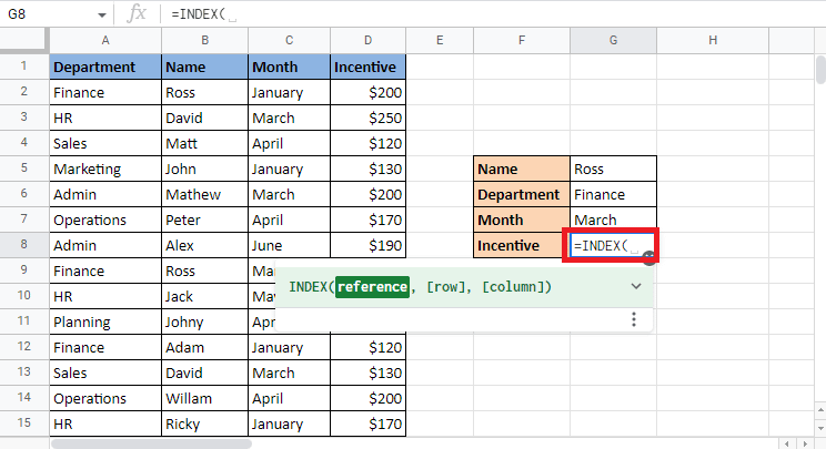
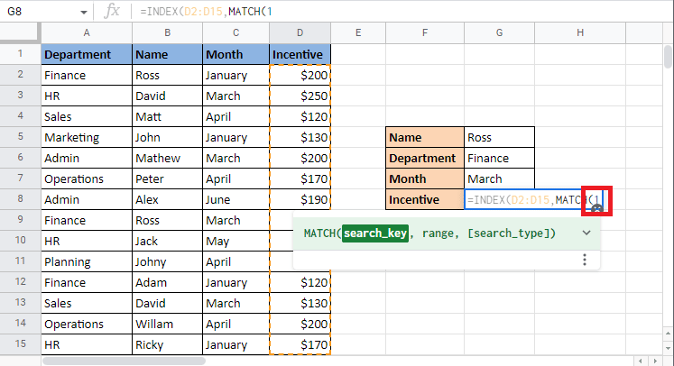
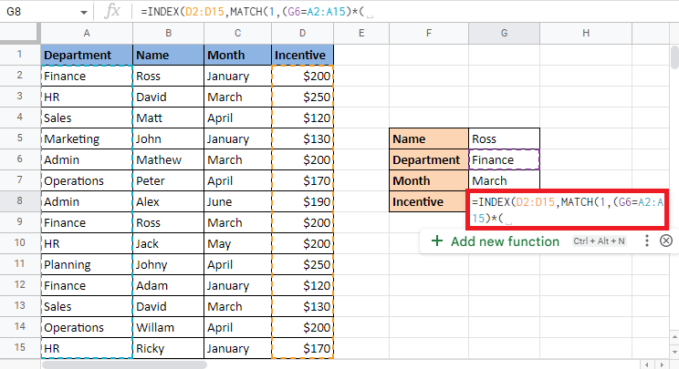
1. Start applying the INDEX MATCH formula in the required cell which is G8 in this case. Begin by typing INDEX.
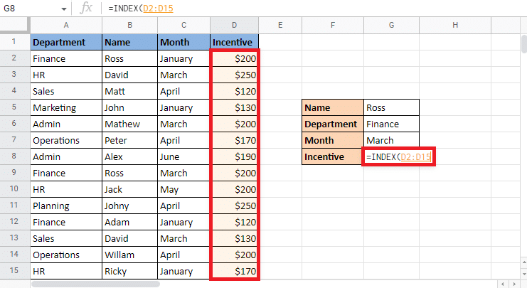
2. For the reference argument, select the Incentive column as it gives the target value.
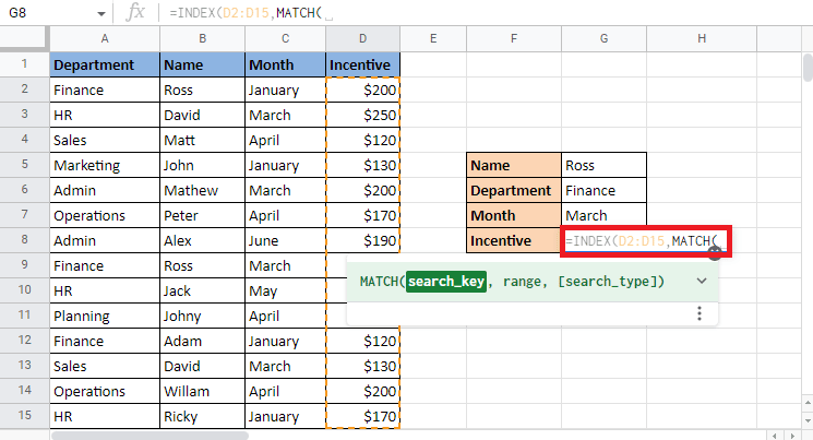
3. Type comma (,) and start constructing the MATCH formula.
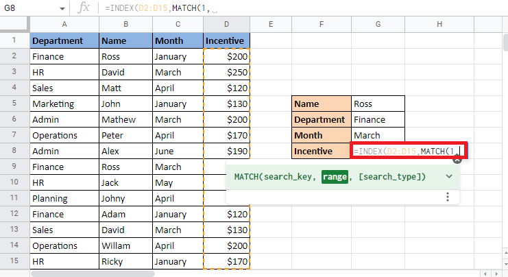
4. Enter the search_key as 1 as explained in the index match multiple criteria syntax Google Sheets.
5. Add comma (,) to move to the next argument of adding criteria to make matches.
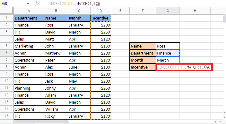
6. Open brackets and choose the first criteria to match which is the department. Select the Finance cell which is in cell G6.
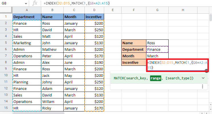
7. Put an equal to (=) sign and match it to the column by selecting the department column. Then close the brackets.
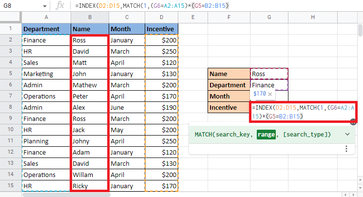
8. Put an asterisk (*) and open brackets to enter the next criteria.
9. Select the next reference cell G5 which is the Name Ross, put an equal to (=), select the Name column, and close the brackets.
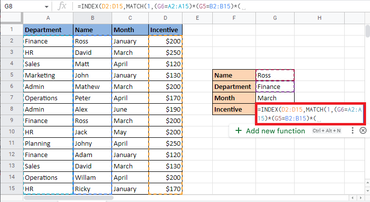
10. Put an asterisk (*) and open the brackets for the last criterion which is the Month.
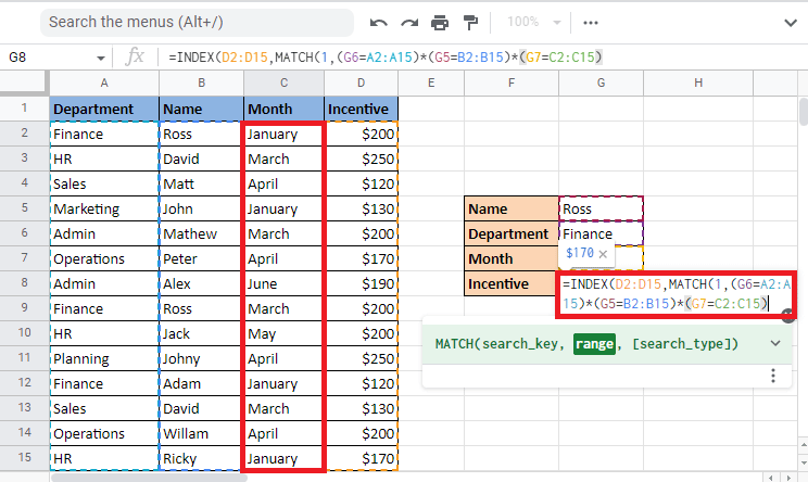
11. Select the reference cell G7 which is the month of March, put an equal to (=), select the Month column, and close the brackets.
12. Add comma (,) and type 0 to get the exact match.
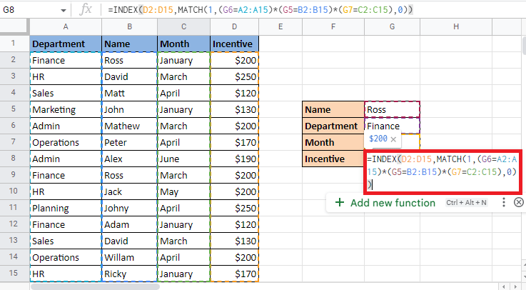
13. Close the bracket twice to complete the MATCH formula and the INDEX formula.
14. Press Enter key to get the target value.
Also Read: How to quickly wrap text in Google Sheets?
Can You Use INDEX MATCH Across Multiple Google Sheets?
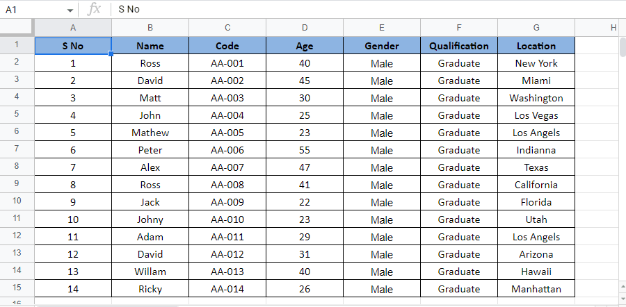
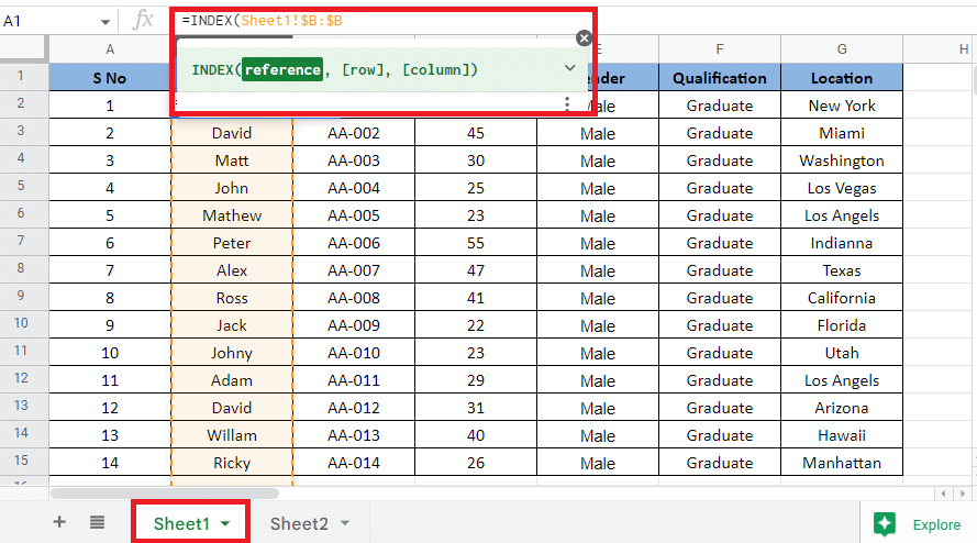
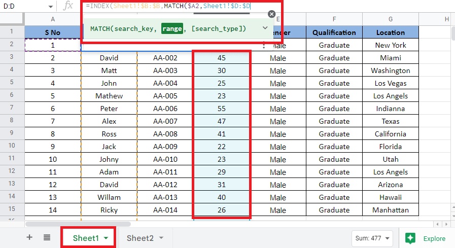
Yes, INDEX MATCH is the best option if you are wondering how to use data across multiple Google Sheets. In this case, we will be using two sheets. The first sheet contains details of employees such as the code, gender, qualification, gender, and location.
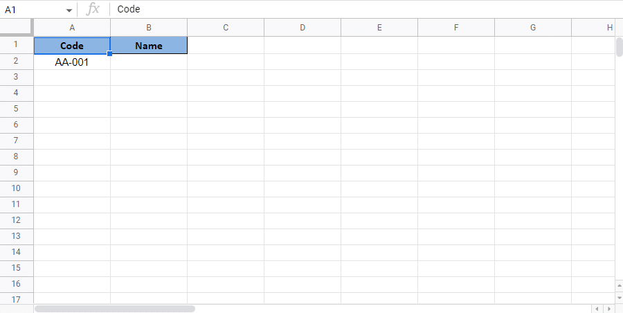
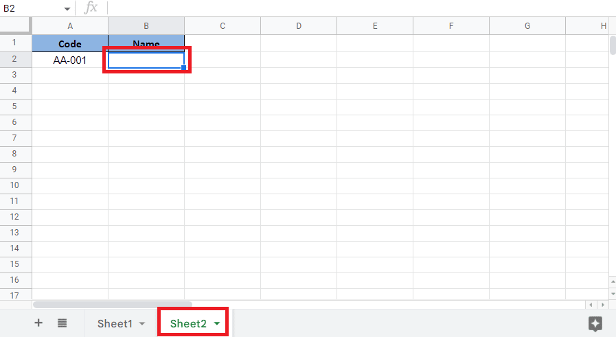
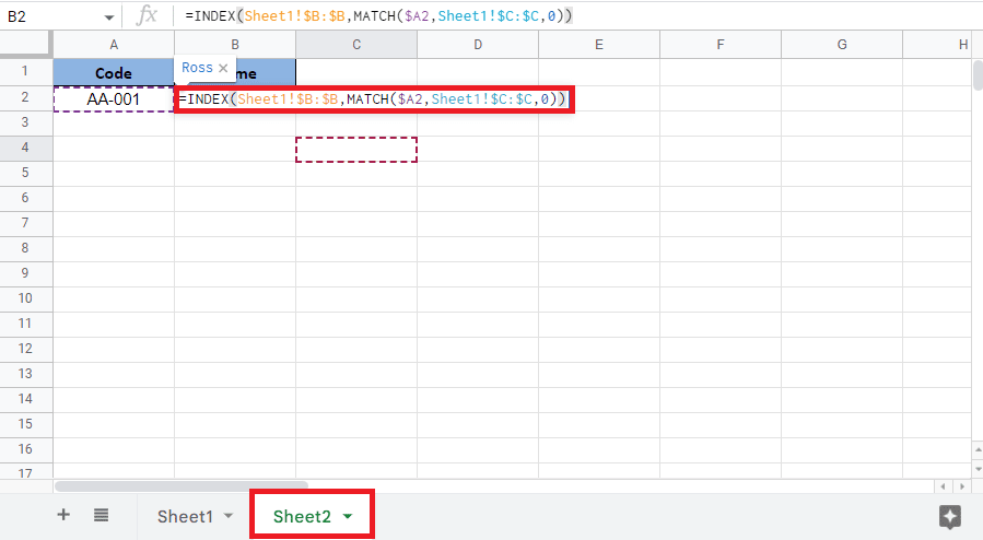
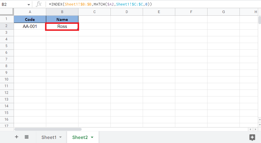
In the second sheet, we will find out the employee details using their code by applying the INDEX MATCH formula across the sheets.
Let’s begin with steps to see can you use INDEX match across multiple Google Sheets:
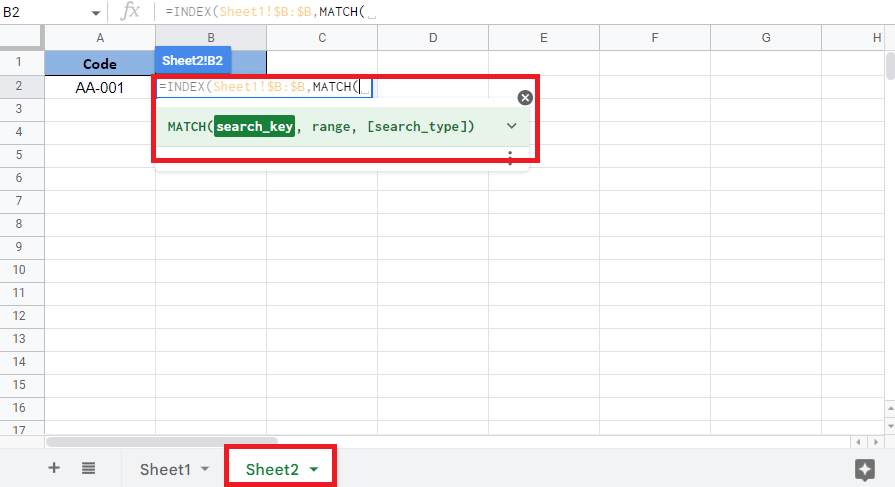
1. Select the cell in which you want to get the target value in Sheet 2. In this case, we will be selecting the B2 cell.
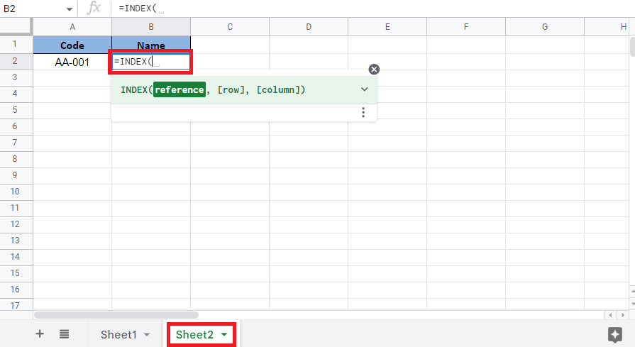
2. Start with an equal to (=) and type the INDEX formula.
3. For the reference argument, go to Sheet1, select and lock the column by pressing the F4 key.
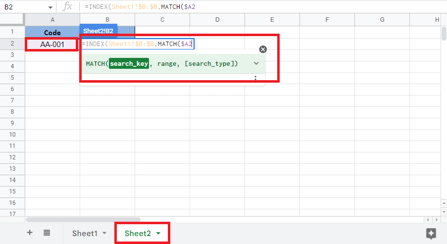
4. Open Sheet2, add comma (,) and start the MATCH function.
5. Select the reference cell A2 to the target value which is the code available on Sheet2 and lock the required cell.
6. Add a comma (,), select the column with the reference cell in Sheet1, and lock the column by pressing the F4 key.
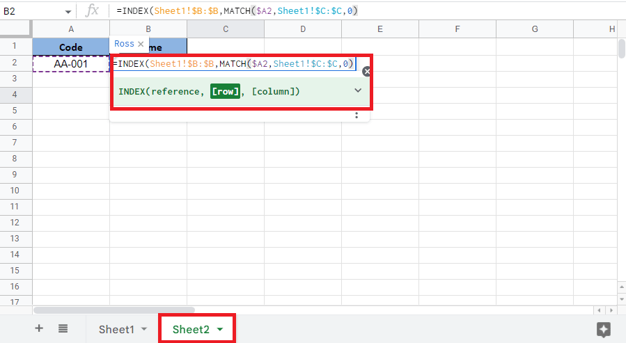
7. Add comma (,), type 0 to get the exact match, and close the bracket to complete the MATCH formula.
8. Close the bracket again to complete the INDEX formula.
9. Press the Enter key to get the target value.
Also Read: 6 ways to remove duplicates in Google Sheets
Frequently Asked Questions (FAQs)
Q1. How many criteria can be used in an INDEX MATCH formula?
Ans. INDEX MATCH as a function was introduced post the introduction of VLOOKUP and HLOOKUP functions. The main purpose of INDEX MATCH is to overcome the limitations of VLOOKUP and HLOOKUP. As we already know that the number of rows and columns used by the INDEX and MATCH functions is more than two. Therefore, we can conclude by saying that infinite criteria can be added when we use the INDEX MATCH function.
Q2. Why should you prefer INDEX MATCH over VLOOKUP?
Ans. Listed below are the reasons why you should consider using INDEX MATCH over VLOOKUP:
- INDEX MATCH starts to look for values from the left side of the column.
- It also keeps into account the text case when necessary.
- This function also gives you a vertical lookup value when used with multiple criteria.
- Adding new rows and columns does not interfere with the existing data.
Recommended:
This article was all about using INDEX MATCH with multiple criteria in and across Google Sheets. We hope that this guide was helpful and you were able to learn how to INDEX MATCH multiple criteria Google Sheets. Let us know which method worked for you best. If you have any queries or suggestions, then feel free to drop them in the comments section below.
